Deciphering Notation: The Maximum Likelihood Estimator
We can unpick many interesting ideas from this equation, used in many areas of supervised learning.

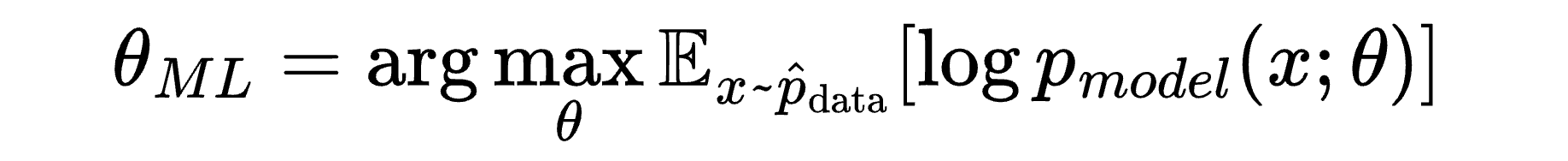
First, the equation:
Next, let’s set up a simple example for connecting abstractions to the real world:
We’re building a model that will tell us how likely it is to rain on a future day.
We pretend that previous weather has no impact on later weather, so our training data points are independent.
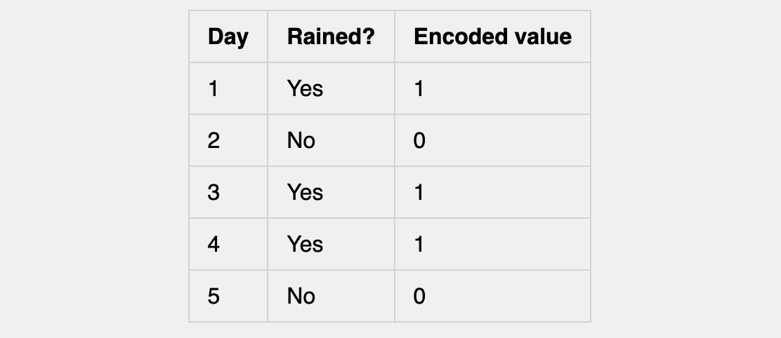
Our training data might look like this:

In other words, we have the training set:

Now we can work through the notation piece-by-piece, using the example to illustrate what each part is doing.
The simplest possible model
The simplest possible model has one parameter, θ, which represents the possibility of rain on any given day:

The semicolon in p_model(x; θ) is just a notation meaning: “This is a function of x, and it’s parameterised by θ” so that different choices of θ give different models.
θ = 0.5 means equal chance of rain or no rain. θ = 0.9 means it’s very likely to rain.
Our task is to pick the best θ, where “best” means the value of θ that makes our actual training data look as likely as possible.
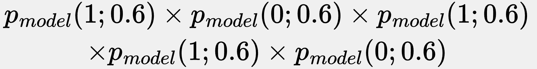
Recall that our simple example training set is:
If we pick θ = 0.6, then our model tells us the probability of seeing the exact sequence {1,0,1,1,0} is:

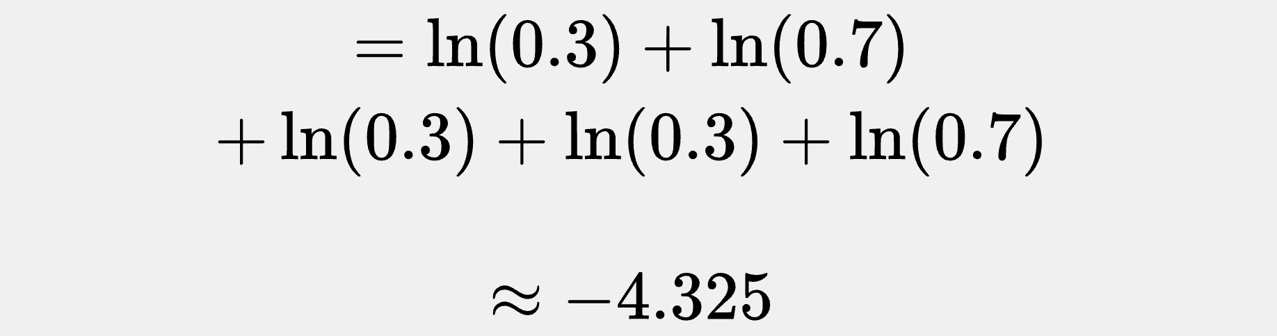
But if we picked θ = 0.3, we’d find ourselves with:

So θ = 0.6 makes our data more likely than θ = 0.3 does.
So we’re looking for the value of θ that maximises this probability which, currently, we’re calculating as a product.
At this point, our “work-in-progress” maximum likelihood estimator looks like this:

Problems with products, solved by logarithms
We notice that, if we had a real-world training set containing a million data points, this product would become extremely small.
It is called “numerical underflow” when numbers become so small they are essentially lost from floating point arithmetic, as they are rounded to zero during computation.
And we also know that we’re using the argmax function, which finds the input that yields the largest output for a given function.
So we think about taking the logarithm of our probability product, because:
The logarithm function turns products into sums, so we won’t multiply tiny numbers until they disappear completely
For numbers between 0 and 1, the closer the number is to zero, the further from zero (in the negative direction) the logarithm will be
More generally, logarithms preserve the order of numbers: If a is greater than b, then log(a) is greater than log(b)
(We’ll use the natural logarithm here.)
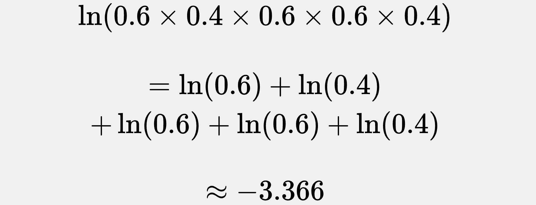
For θ = 0.6, the logarithm of our probability product is:
And if we set θ = 0.3:
Of course, the sum allows us to avoid the multiplication of increasingly tiny numbers.
Our log-probabilities are negative, but higher probabilities become negative numbers that are closer to zero, so argmax can still identify the “best” value for θ without any trouble.
So we’re very happy with this logarithm decision.
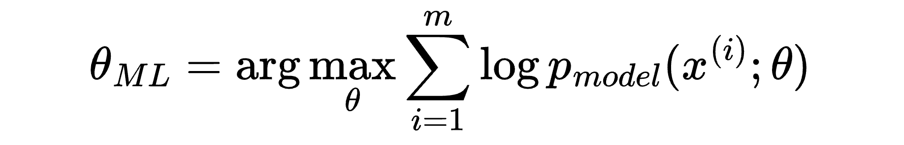
And we can update our “work-in-progress” maximum likelihood estimator to:
Why not take the average?
At this point, we spot a new opportunity.
If we take the average of the log-probabilities for each value of θ by dividing their sum by m, this won’t change the order of the values, either.
So we can update our “work-in-progress” equation to:
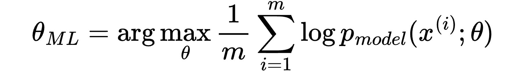
(This is just the first half of the opportunity, so continue on to see the whole thing.)
Next, we consider what would happen if we randomly sampled a data point from our training set to compute the log-probability for, with an equal probability of selecting any one of them.
In other words, we introduce a random variable, X, with probability distribution, p̂_data, to represent a sampled data point and the likelihood of it taking a particular value.
Recalling our simple example training data:

If we pick one of the days at random, with equal probability of picking any day, then the likelihood of picking either a 1 or a 0 is:

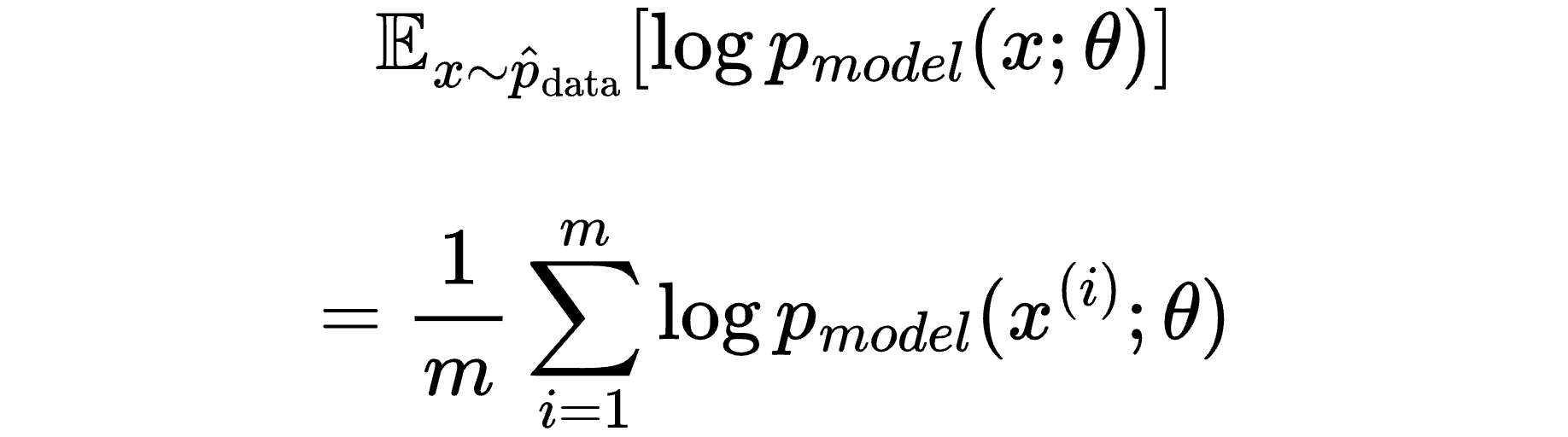
We can then ask what the expected value of the log-probability would be for this sampled data point.
Since expected value is a weighted average of all values a random variable can take, we see that the expected value of the log-probability of a randomly sampled data point would be the average of all of the log-probabilities.
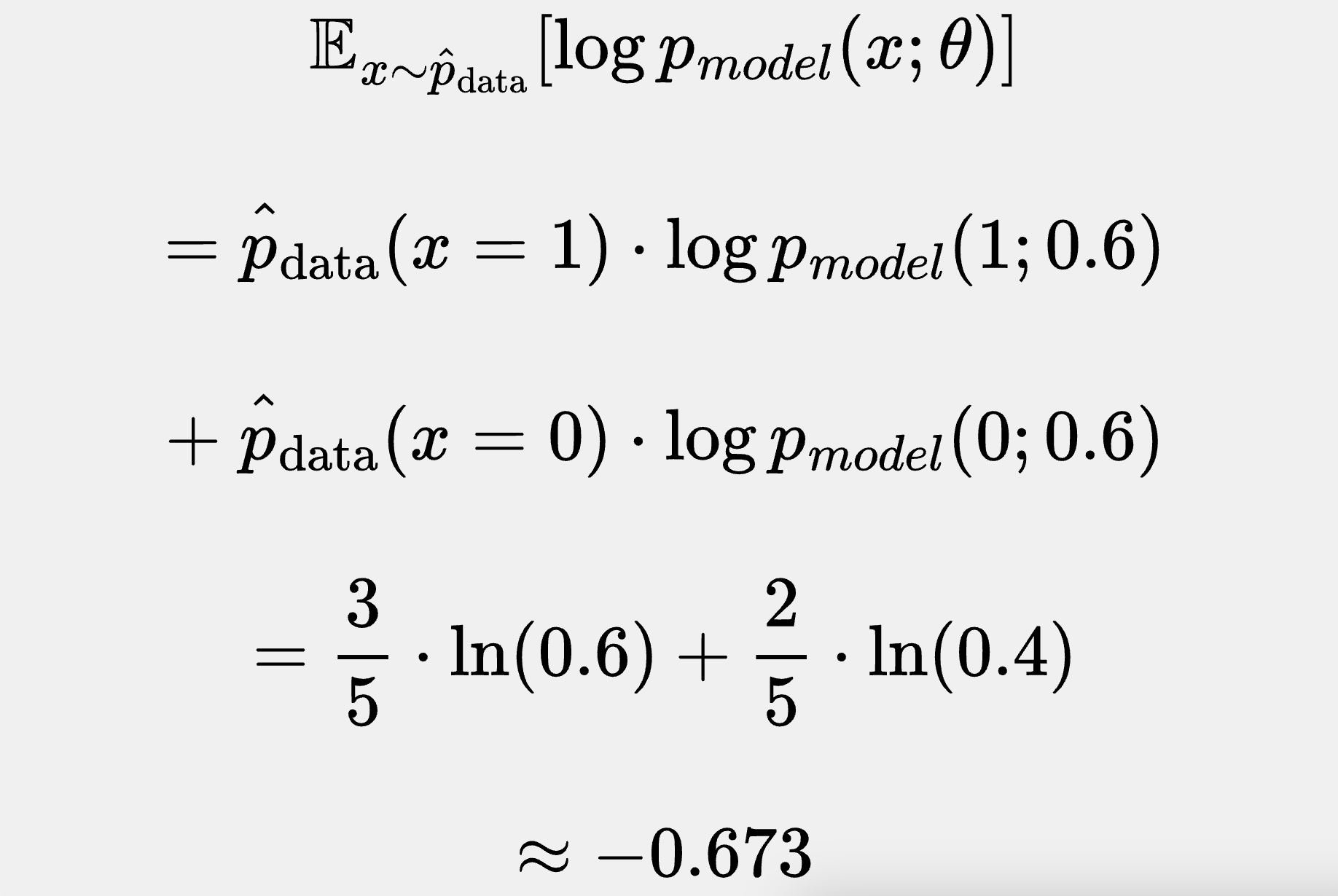
Returning to our example, and choosing θ = 0.6 to see the result for this expected value calculation, we can take a direct look at the log-probabilities first:
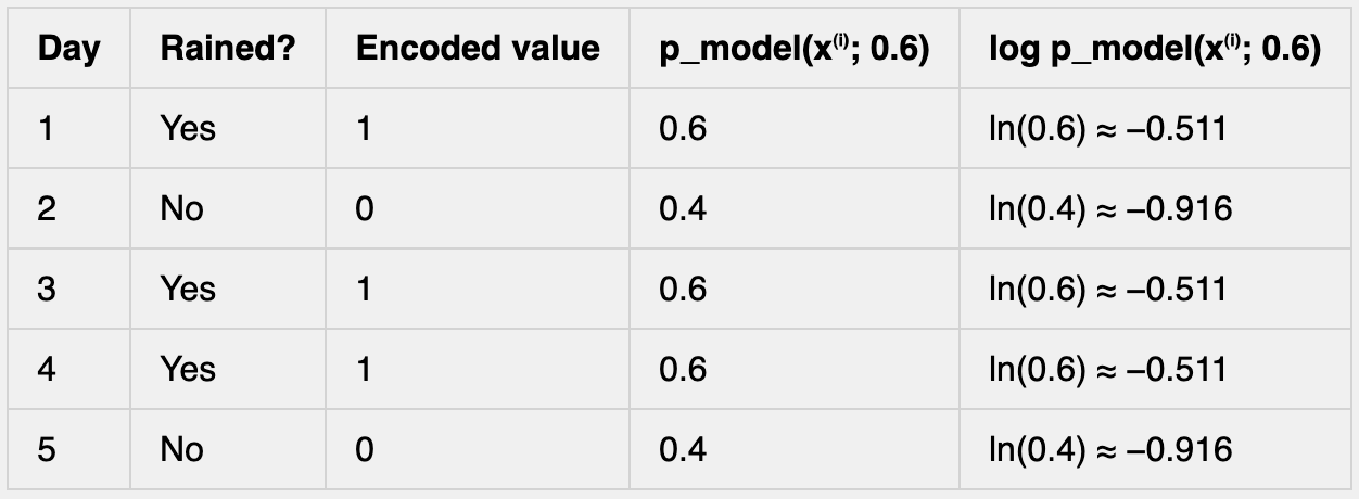
We can sum these log-probabilities and divide by 5, if we want, to obtain approximately -0.673.
And, recalling the likelihoods we saw in the previous example section, we can compare this to the expected value weighted average calculation:
That is to say:
So the expected value of the log-probability for a randomly sampled data point equals the average of the log-probabilities. Interesting!
And not only interesting but significant, because p̂_data is an empirical distribution that becomes a better approximation of the true distribution, p_data, as the training data set grows. This is the law of large numbers.
And p_data is what we really want to model (although we can never do so perfectly).
So we swap this expected value into our “work-in-progress” equation:

But we have, in fact, arrived at the “real” equation. So we can remove the “work-in-progress” label, and pause to appreciate our progress (and the equation itself).
Time for a cup of tea ☕️